How to learn quantum computing: a practical beginner roadmap from first circuit to evidence.

Quantum computing looks harder than it needs to because learners often meet linear algebra, physics notation, Python, cloud accounts, hardware noise, and algorithm claims at the same time. Separate those layers. Begin with one question: can a two-qubit Bell circuit produce strongly correlated measurements in the ideal model?

A complete first attempt has six actions: predict, build, inspect, simulate, explain, and save. QFlow Studio and QFlow Academy can provide a browser-based visual route without a local SDK installation, subject to the access available to the learner. IBM Quantum Learning and the official Qiskit documentation provide the authoritative theory and SDK path. These resources play complementary roles; an ecosystem reference does not imply an endorsement.

For a first Bell workflow, you need comfort with binary values, simple probability, the idea of a coordinate or vector, and following operations in order. You do not need calculus, advanced quantum mechanics, or a proof of every result before touching a circuit. Complex numbers, vectors, matrices, tensor products, and eigenvalues become important as you move from circuit literacy to derivations and algorithms.

Python is optional for the no-local-install QFlow path. For the local Qiskit path, the practical minimum is being able to create a virtual environment, install a package, run a notebook or script, read a function call, and inspect a dictionary of counts. Learn loops, functions, imports, and basic debugging alongside the quantum exercises; do not postpone all circuit work until you consider yourself a Python expert.

A qubit is the basic information system described by a normalized quantum state. Relative to a chosen measurement basis, that state has amplitudes associated with possible outcomes. It is not simply a classical bit whose value is hidden. A gate is a controlled transformation of that state; common circuit gates are represented by unitary operations, while measurement is a different kind of operation.

Superposition means a state can be a linear combination of basis states. It does not mean a measurement displays two classical answers at once. Entanglement means a multi-qubit state cannot be described as independent states for each qubit; the Bell workflow makes that joint structure visible through correlated results.

Interference occurs because amplitudes have phase and can reinforce or cancel when quantum paths are recombined. Useful algorithms shape amplitudes before measurement; they do not merely try every answer and read all of them. Measurement converts a quantum state into a classical outcome in a chosen basis, so repeated circuit executions—shots—are used to estimate a distribution.

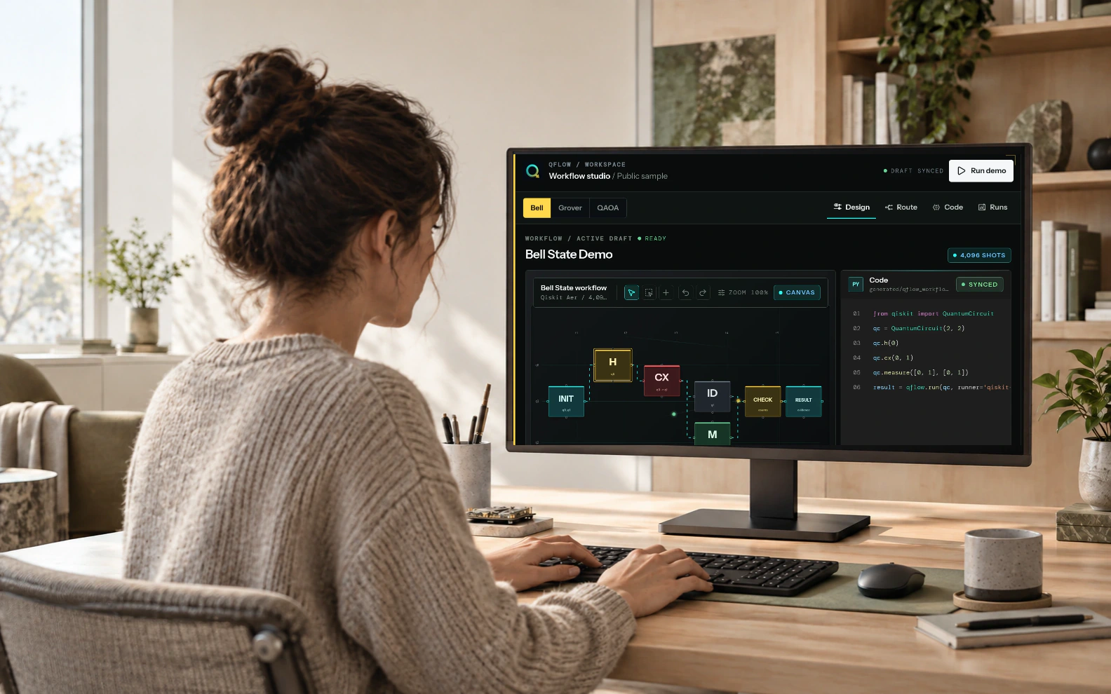
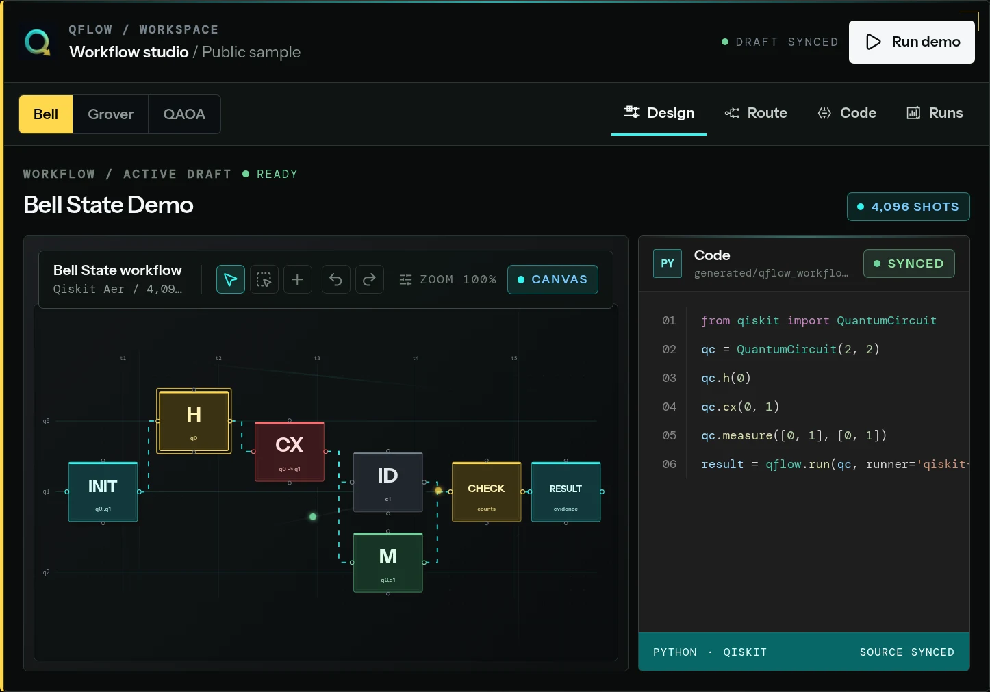
The no-local-install QFlow route starts on a visual canvas: place operations, trace the wires, inspect generated Qiskit or OpenQASM, run an available simulator route, and keep the attempt with its result. This reduces local setup friction while keeping the source visible. It is appropriate for first contact, classrooms, demonstrations, and learners who want a circuit-level mental model before managing Python packages.

The local Qiskit route starts with a fresh Python virtual environment and the current packages specified by IBM’s installation and quickstart guides. It is appropriate when you want to write and test source directly, integrate notebooks with data analysis, use SDK APIs, or eventually prepare workloads for a provider. Do not copy an old installation command or tutorial version without checking the current official page.

These routes should converge. A visual learner should inspect and eventually edit source; a code-first learner should draw circuits and explain every operation. QFlow is an accessibility and evidence layer, not a replacement for Qiskit, IBM Quantum infrastructure, or foundational instruction.

Minutes 0–5: write the question and prediction before opening a tool. Use: ‘After H on q0 and CX from q0 to q1, an ideal measured Bell circuit should return only 00 and 11, with an approximately even distribution over many shots.’

Minutes 5–15: create two qubits, apply H to the first, apply controlled-X with q0 as control and q1 as target, then measure both. Build it visually in QFlow or follow the current IBM Qiskit quickstart locally. Inspect the gate order and the generated or handwritten source before execution.

Minutes 15–25: run about 1,024 simulator shots and inspect the counts. A result such as 526 occurrences of 00 and 498 of 11 is plausible; another run will differ. In an ideal simulation, 01 and 10 should be absent. Minutes 25–30: save the circuit, shot count, raw counts, expected distribution, and a two-sentence interpretation.

The two-qubit register begins in 00. H on q0 creates an equal-amplitude superposition for that qubit. The controlled-X then flips q1 only on the branch where q0 is 1, producing the Bell state commonly written as (|00⟩ + |11⟩)/√2. Measuring both qubits therefore produces correlated bit strings.

The ideal probability model assigns one half to 00, one half to 11, and zero to 01 and 10. Finite-shot sampling does not promise exactly 512 and 512 at 1,024 shots. The acceptance check is that the observed distribution is reasonably close to the expected structure for the selected simulator and shot count—not that one random sample matches a perfect split.

On a noisy device, 01 and 10 can appear and the dominant probabilities can shift. Those differences do not automatically demonstrate useful quantum behavior or a broken circuit. They create a new investigation involving transpilation, device topology, gate and readout errors, calibration context, and comparison with an explicit simulator baseline.

Repeat the Bell circuit until you can reconstruct it without copying. Then remove CX and predict the difference: q0 varies while q1 remains fixed. Restore CX, add X to one qubit at a declared point, and predict which bit strings should appear. For every variation, keep the prediction beside the counts.

Open the Qiskit and OpenQASM views and map each visual operation to one source instruction. Change one gate and find the exact code difference. Finish the day by explaining qubit, gate, superposition, entanglement, interference, measurement, basis, and shot in your own words, using the circuit as the example rather than reciting definitions.

Days two and three should cover basis states, X, H, Z, CX, measurement, shots, and simple statevector or sampling views. Use tiny circuits to see that Z can change phase without directly changing computational-basis counts, then use a later H to turn that phase difference into a measurable interference effect.

Days four and five should connect the same circuits to Qiskit source. Create a clean environment if you began visually, reproduce the Bell workflow from the official quickstart, draw the circuit, inspect counts, and record package versions. If you began in code, rebuild the same experiment visually and explain the block-to-source mapping.

Days six and seven should introduce one small algorithmic pattern, such as a two-qubit Grover example, only after the learner can identify preparation, oracle, interference or amplification, and measurement. Keep the scale, simulator route, baseline, and learning claim explicit. A toy example teaches mechanics; it does not prove speedup or business value.

Days 1–7 — circuit literacy: complete Bell and several one-change experiments; explain the six core concepts; map every block to source; keep a small result record. Exit criterion: you can predict and explain simple one- and two-qubit distributions.

Days 8–14 — code literacy: install Qiskit in a dedicated environment, reproduce the visual circuits in Python, draw them, sample them, and handle basic errors. Learn vectors, complex amplitudes, matrices, and tensor products alongside the code. Exit criterion: you can build and debug a small circuit without blindly copying a notebook.

Days 15–21 — workflow literacy: study IBM’s map–optimize–execute–post-process pattern, add a small Grover or parameterized example, define a baseline, and record inputs, versions, shots, output, and limitations. Exit criterion: another learner can reconstruct your simulator experiment from the saved record.

Days 22–30 — route literacy: decide whether your question needs hardware. If it does, review account, credential, cost, queue, target, transpilation, and privacy boundaries before a small QPU run. If it does not, deepen simulation, mathematics, or an application domain. Exit criterion: you can justify the route and describe what the result does and does not establish.

A QPU is justified when you need to study physical noise, connectivity constraints, transpilation for a target instruction set, calibration-sensitive behavior, execution queues, or provider-specific runtime characteristics. Before submitting, the circuit should already pass its ideal or declared noisy-simulator checks and the team should know what new evidence the hardware run can provide.

A QPU is usually unnecessary for learning gate syntax, debugging a logical circuit, checking an ideal Bell distribution, or demonstrating a toy algorithm. Real hardware does not make a weak experiment meaningful. It adds constraints, variability, account requirements, queue time, and possibly cost. Review the current IBM account and hardware documentation rather than assuming access or credits.

Do not run first and invent an explanation afterward. Write the expected outcomes and failure conditions before execution. Do not interpret superposition as seeing every answer, entanglement as faster-than-light messaging, or a noisy histogram as proof of advantage. Do not expect a finite-shot Bell run to split exactly fifty-fifty.

Avoid copying stale Qiskit code into a mixed Python environment, changing several circuit elements at once, hiding generated source behind a visual interface, or moving to hardware before the simulator behavior is understood. Also avoid starting with QAOA, quantum machine learning, or error correction simply because the vocabulary sounds advanced; choose the next topic because it exercises a capability you are ready to inspect.

A beginner record should contain the question, prediction, circuit, source representation, simulator or provider route, package or tool context, shot count, raw counts, interpretation, limitation, and next change. Preserve failed attempts when they explain a correction. This makes feedback specific: an instructor or teammate can comment on the prediction, gate order, source, run configuration, or conclusion.

QFlow Academy can connect lesson framing, runnable labs, attempts, feedback, and reviewer-safe completion evidence. A certificate should point to declared completion criteria, not imply universal competence. Private student information, credentials, billing data, and administrative notes stay outside a shared evidence packet.

If you cannot explain Bell counts, repeat the first-day experiments and strengthen probability and basis-state reasoning. If the visual circuit makes sense but the source does not, continue with the visual Qiskit and OpenQASM guide. If code runs but route choice is unclear, study simulator-versus-QPU routing. If another person cannot reconstruct the experiment, study workflow lifecycle and reproducibility before adding complexity.

If you can predict, code, simulate, and document small circuits, choose one bounded next problem. Use Grover to study an oracle and interference pattern. Use a small QAOA exercise only when you can define the classical objective, parameters, sampling method, and baseline. Use a university lab programme or assessment rubric when the next problem is teaching a cohort rather than advancing one learner.

IBM Quantum Learning supplies official modules with background, Qiskit code, practice questions, and optional video material. IBM’s Qiskit quickstart, installation, Composer, development-pattern, and hardware guides provide current primary instructions. QFlow Studio connects visual construction, generated source, run context, and evidence; QFlow Academy connects those workflows to attempts and feedback.

Universities and teams should define prerequisites, accessible simulator routes, instructor support, assessment rules, privacy boundaries, and explicit hardware gates before launching a cohort. Neura Parse’s quantum workflow service can help frame programmes and pilots around questions, reusable workflows, and evidence. Any IBM-related roadmap language must remain accurately scoped; references to IBM Quantum and Qiskit do not by themselves establish formal partnership, endorsement, bundled access, or credits.